Lakehouse Essentials: building a Databricks medallion stack as a one-person data team

Building a lakehouse sounds like a daunting engineering task. It’s a phrase that summons images of a full platform team, months of infrastructure yak-shaving, and a budget line that makes finance wince. I wanted to write up the fundamental components I actually used to build a lakehouse on Databricks at GetGo — and along the way show that, for a single-person data operation, it’s genuinely more tractable than the marketing suggests. The reason is simple: Databricks bundles most of the hard parts out of the box, so one person can spend their time on data processing rather than infrastructure. You’ll soon see that it’s really easy. Let’s go.

(A note on dating: this is written up as it stood in early 2025. It reflects the tooling and the one-team context at GetGo at the time, and some of it — especially the platform speculation — has already moved on. Read it as field notes from a specific moment, not a current-state reference.)

The whole thing comes down to three sections: ETL, Delta Lake, and Orchestration.

The shape of the thing: medallion architecture

At a high level, we build the lakehouse on Delta Lake, and organise it into three “zones”:

• a raw zone for landing and processing incoming files,
• an enrichment zone that extracts transactional data, cleans it, and stores it as facts and dimensions,
• an aggregation zone that builds business-level summaries.

This is the medallion architecture — Bronze, Silver, Gold — named so the tiers are easy to refer to and reason about. Bronze is raw and trusting of nothing; Silver is clean, typed, and business-shaped; Gold is aggregated and ready for a dashboard.

Medallion architecture — the Bronze, Silver and Gold tiers.

The three lakehouse zones, and how access is fenced off between them.

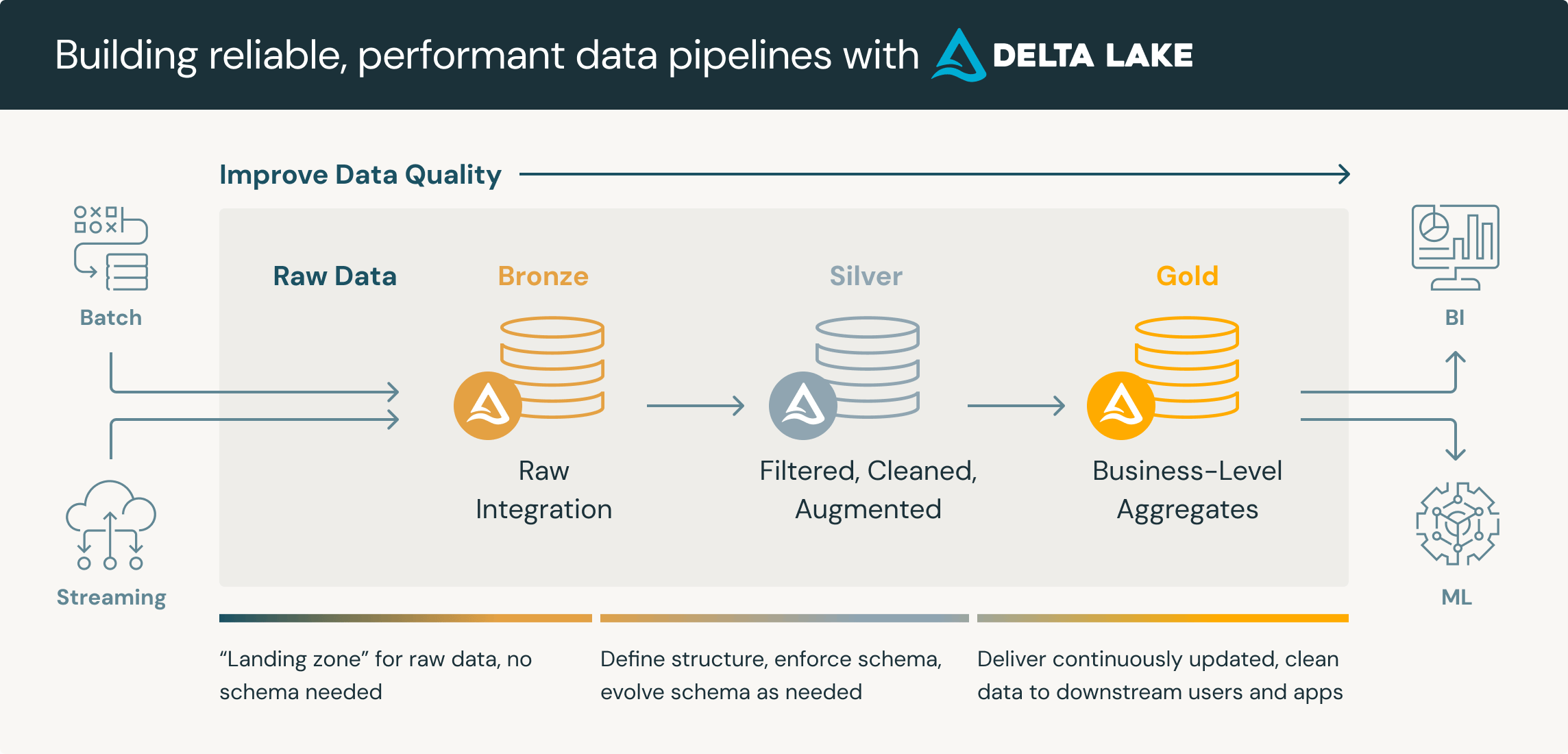
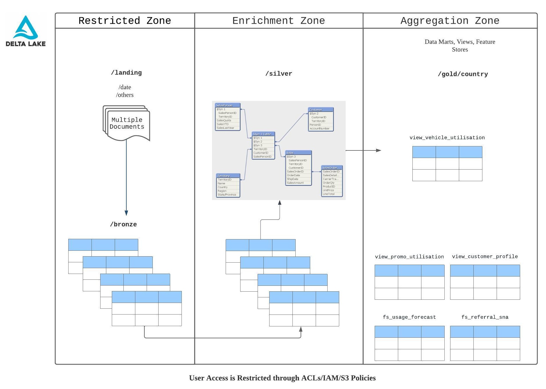
The unified platform is what makes the one-person version viable. Out-of-the-box features — streaming ingestion, incremental change tracking, ACID tables, a built-in scheduler — amplify what a single data engineer can carry.

ETL

Data ingestion

The first step is ingestion: think of it as continually producing files of incremental data that need to be processed and stored in the warehouse. Those files get generated and dropped into cloud object storage, and from there the lakehouse takes over.

This is probably the hardest and most uncertain part of the whole lakehouse. Data comes from everywhere — email, relational databases, SFTP, documents, accounting software, CRMs, Excel sheets, customer chat platforms, REST APIs, server logs, social media, marketing platforms. The list genuinely goes on. Assuming each source maps to a validated business use case, our job as data engineers is to pipe it in, and the sky’s the limit on how.

Roughly, the toolbox splits into scripts and products:

Scripts

• Python on serverless (AWS Lambda, Azure Functions) or on servers — good for SFTP, social media, and REST APIs
• Google Apps Script — handy for email attachments when your mailbox is Gmail
• SQLAlchemy

Products

• Fivetran, Airbyte, Stitch, Power Automate, AWS Database Migration Service, Estuary, Informatica

The capability of each product, and the combinations of script-and-product you can pull off, are endless. In the end it reduces to a function of cost and the environment you operate in. If you’re not on Gmail, for example, you’ll need an email connector (Fivetran, Airbyte) or you’ll stand up AWS Simple Email Service to save attachments into S3 — and that S3 bucket should sit in a sanitisation zone so anti-virus can scan files before they ever reach the lakehouse.

For the mechanical SFTP→S3 problem, I have an older step-by-step that pairs the AWS CLI, a Makefile, and Python to move files into object storage. I wrote it in 2017 and it was still working in 2024 — a small testament to how boring and reliable the right ingestion plumbing should be.

Relational databases

For databases, I’ve used Fivetran and AWS DMS to perform Change Data Capture (CDC). They behave differently in a way that matters:

• Fivetran ships Teleport Sync, which pulls deltas without requiring you to enable binary logging on the source database.
• AWS DMS relies on the bin log to identify changes. The bin log degrades database performance from an IOPS perspective, but in our case the pros outweighed the cons.

A platform-specific wrinkle: Fivetran can push straight into your Bronze tables, whereas AWS DMS drops CSV/Parquet into a landing S3 bucket that then needs processing into Bronze. One integration point of friction, saved.

Databricks had also just acquired Arcion, a CDC specialist, and with Unity Catalog leaning on Lakehouse Federation, my then-hope was that native CDC replication into the lakehouse would become table stakes and pull ingestion inside the platform. Time will tell on that one.

Data processing

Bronze — the raw / ingestion zone

Files are now sitting in object storage. Autoloader does exactly what its name says: it automatically reads new files as they land, using Spark Streaming, and keeps a log of which files have already been ingested so the incremental pattern is reliable. New arrivals are picked up and loaded into a streaming DataFrame ready for processing.

For each source we keep two notebooks: one to initialise the Bronze table from everything currently in object storage, and one to process the incrementals (deltas). The init notebook just reads all the files that exist today and forms the initial raw table.

One deliberate choice when creating Bronze: cast every column to String. You’re not fighting messy type inference at ingestion; you’re just forming a structured table so cleaning can proceed. Real types come later, in Silver.

Once the Bronze table exists, it’s ready to take deltas via Autoloader. Reading a new batch into a Spark DataFrame:

bronze_booking_concluded_df = (
    spark.readStream
    .format('cloudFiles')
    .option('cloudFiles.format', 'csv')
    .option('header', 'true')
    .option('inferSchema', 'true')
    .option('cloudFiles.schemaLocation', schema_path)
    .option('rescuedDataColumn', '_rescue')
    .load(input_table_path)
)

New files are picked up at the next scheduled run. If a source adds new columns you didn’t plan for, Autoloader doesn’t blow up — the surprises land in a _rescue column as JSON, so the pipeline keeps flowing while you decide what the new field means. Then you append into the Bronze table:

(
    bronze_booking_concluded_df
    .writeStream
    .format('delta')
    .trigger(availableNow=True)
    .option('mergeSchema', 'true')
    .option('checkpointLocation', checkpoint_path)
    .outputMode('append')
    .start(output_table_path)
    .awaitTermination()
)

availableNow=True is the key operational trick: it processes all currently-available data and then exits, instead of running forever. That lets you schedule the Delta notebook as a batch job at fixed times. If you truly want continuous ingestion, you leave a cluster running 24/7 and drop the bounded trigger.

Silver — the enrichment zone

Silver tables are built from Bronze, and again each gets an init and a delta notebook. The init reads Bronze wholesale, but this time selects only the columns you want and casts them into proper types — strings become dates, integers, and so on — and removes duplicates. This is where raw text becomes trustworthy data.

The delta notebooks lean on Spark Streaming plus Delta Lake’s Change Data Feed to process only what’s changed since the last known point. (Practical note: don’t use Databricks’ own docs for CDF — go to the Delta Lake docs, they’re clearer and have better examples.)

Concretely, ingesting from a Bronze table created by AWS DMS CDC. upsertToDelta is the micro-batch function Spark Streaming calls to apply the deltas — “upsert” being Update/Insert/Merge in one, which is one of the genuinely nice Delta features. Without it you’d stage the incremental data in a temp table and then merge the staging table into the target by hand.

def upsertToDelta(microBatchOutputDF, batchId):
    (
        delta_table.alias("target")
        .merge(
            (
                microBatchOutputDF
                .filter(col('Op').isin(['I', 'U']))
                .withColumn(
                    'rnk',
                    rank().over(
                        Window.partitionBy(f'{join_key}')
                              .orderBy(col('transact_id').desc())
                    )
                )
                .filter(col('rnk') == 1)
                .drop('rnk')
                .dropDuplicates()
            ).alias('source'),
            f'source.{join_key} = target.{join_key}'
        )
        .whenMatchedUpdateAll(condition=update_condition)
        .whenNotMatchedInsertAll()
        .execute()
    )

(
    silver_booking_concluded_delta_df
    .writeStream
    .format('delta')
    .foreachBatch(upsertToDelta)
    .outputMode('update')
    .trigger(availableNow=True)
    .start()
    .awaitTermination()
)

Why all the Window / rank() ceremony? Because plain dropDuplicates() in Spark doesn’t keep the latest or earliest row — it drops duplicates arbitrarily. If a key arrives several times in a micro-batch, you want to deterministically keep the newest one by transact_id, so you rank within the partition and keep rank 1. It’s the difference between “mostly correct” and “defensible at 2am when someone asks why the numbers moved.”

If the data genuinely doesn’t care about row order, you can skip the windowing and keep it simple:

def upsertToDelta(microBatchOutputDF, batchId):
    (
        delta_table.alias('t')
        .merge(
            microBatchOutputDF.dropDuplicates([join_key]).alias('s'),
            f's.{join_key} = t.{join_key}'
        )
        .whenMatchedUpdateAll()
        .whenNotMatchedInsertAll()
        .execute()
    )

(
    fact_c_delta_df
    .writeStream
    .format('delta')
    .foreachBatch(upsertToDelta)
    .outputMode('update')
    .trigger(availableNow=True)
    .start()
    .awaitTermination()
)

Silver — fact and dimension tables

The whole point of the warehouse is to make information easy to analyse. Transactional databases aren’t built for that: they’re heavily normalised to preserve data integrity, which is great for OLTP and miserable for analytics. Fact and dimension tables are de-normalised — shaped for aggregation and, ultimately, dashboards that answer real business questions. This master data also preserves the business context that downstream teams rely on.

A few principles that keep the semantic layer humane:

• Enrich with data from outside the transactional system — weather, for instance — to widen the range of questions the model can answer.
• Replace numeric category references with the category names, so you shed unnecessary joins.
• Keep infrequently-used reference data separate and join it only when needed.

Each fact and dimension table gets its own init and delta notebooks, same as everything else. We also keep quarantine tables for records that fail quality or integrity checks. The value is that a workflow can continue running while bad rows are isolated and fixed before re-introduction — at the cost of an extra daily check that the quarantine batches are actually being worked.

The classic enrichment dimension is dim_dates. Here’s how I generate a calendar and shape it into a usable dimension (modified from a find on Stack Overflow, no shame):

begin_date = '2021-01-01'
end_date   = '2030-12-31'

(
    spark.sql(
        "select explode(sequence(to_date('%s'), to_date('%s'), interval 1 day)) "
        "as calendar_date" % (begin_date, end_date)
    )
    .createOrReplaceTempView('dates')
)

Then a SQL pass adds the calendar attributes:

create or replace temporary view temp_silver_dates as (
  select
    calendar_date,
    year(calendar_date)  as year,
    month(calendar_date) as month,
    lower(date_format(calendar_date, 'MMMM')) as calendar_month,
    day(calendar_date)   as day,
    lower(date_format(calendar_date, 'EEEE')) as calendar_day,
    weekday(calendar_date) + 1 as day_of_week,
    case when weekday(calendar_date) < 5 then 'Y' else 'N' end as is_week_day,
    case when calendar_date = last_day(calendar_date) then 'Y' else 'N' end as is_last_day_of_month,
    dayofmonth(calendar_date) as day_of_month,
    dayofyear(calendar_date)  as day_of_year,
    weekofyear(calendar_date) as week_of_year_iso,
    quarter(calendar_date)    as quarter_of_year
  from dates
)

Finally we materialise the Delta dimension, deriving week boundaries and left-joining a public-holiday table so analysts get is_public_holiday for free:

spark.sql(f'''
    create or replace table {target_catalog}.{silver_dim_date.schema}.{silver_dim_date.table}
    using delta
    select
      calendar_date, year, month, calendar_month, day, calendar_day, day_of_week,
      is_week_day, day_of_month, is_last_day_of_month, day_of_year,
      week_of_year_iso, quarter_of_year,
      date_sub(calendar_date, day_of_week - 1) as week_start,
      date_add(calendar_date, 7 - day_of_week) as week_end,
      if(h.holiday_date is null, 'n', 'y')     as is_public_holiday
    from temp_silver_dates d
    left join {target_catalog}.{silver_dim_public_holiday.schema}.{silver_dim_public_holiday.table} h
      on d.calendar_date = h.holiday_date
''')

Gold — aggregates

Gold is the summarisation layer: grouping individual quantitative records into categorical aggregates. “What’s the total sales of all retail stores in the North in December?” — that’s an aggregate function (sum, mean, average) applied over fact data and grouped by dimension data.

One design decision to make consciously: view or physical table? If the data is volatile or you want the number always current, a view that computes the summarisation on read can be right; if the aggregate is expensive or point-in-time stable, a physical table that receives appends is often cheaper to serve. The temporal nature of the data decides it.

Delta Lake

Delta Lake is the open-source storage layer the whole thing sits on — the best one-liner for it is parquet files on steroids. Three features do most of the heavy lifting here (and there are many more — the Delta docs have clearer, richer examples than any single post can).

Change Data Feed (CDF)

CDF is what lets each medallion tier consume incremental data efficiently off the tier below. Enable it deliberately, not by default — you’ll find tables where it isn’t needed, so turn it on per-table where you actually stream changes. Combined with Spark Streaming and Delta’s upsert/merge, CDF is the backbone of doing CDC entirely inside the lakehouse.

Time Travel

Time Travel lets you read a table as of an earlier version or timestamp, with roughly a year of history retained. This is unglamorous until it saves your week: we had production customer data accidentally deleted, and because the incrementals had also mirrored the deletion into the lakehouse, we recovered both the production system and the Delta table from a version before the delete. It’s a safety net you won’t appreciate until you need it.

Liquid Clustering

Liquid Clustering improves on manual partitioning and Z-ORDER by simplifying layout decisions to optimise query performance — and crucially it lets you redefine clustering columns without rewriting existing data, so layout evolves alongside analytic needs. In practice, it removes a whole class of “go optimise your tables” chores. We were still applying it to a few multi-terabyte tables at the time of writing.

Orchestration

The line that matters most: planning your update cadence is directly proportional to your spend on Databricks. Tight budget, low urgency? Run weekly. Fast decisions that need fresh numbers? Hourly, or every three or six hours. Cadence is a cost dial, and you should be turning it on purpose.

Databricks Workflows comes out of the box and is the de-facto scheduler on the platform — no separate orchestration infra to deploy or maintain. (You’ll know the alternatives: Apache Oozie, Airflow, Dagster.) The one honest caveat: orchestration reaches within the platform well, but ingestion still lives mostly outside it — a gap I hoped the Arcion acquisition would shrink.

Three things to get right when scheduling jobs:

Compute. Three types — Serverless, Job Compute, and All-purpose. Prefer a shared Job Cluster: it cuts overall cost and ships with Photon enabled by default, so you pay less for more. For irregular, infrequent jobs, try Serverless. For All-purpose clusters, actually look at the compute metrics to find the bottleneck and tune to it.

Number of jobs. As sources and tables multiply, job count grows, a single workflow stops being enough, and you start nesting workflows inside larger ones. That’s where cluster-driver problems surface. The easy path out is Serverless. The hands-on path is disciplined trial and error: grow the driver size, add worker nodes, or fall back from Spot to On-demand — but change one thing at a time so you learn which lever actually worked.

Dependency planning. Your warehouse design dictates which jobs depend on which. Build a core workflow that cannot be allowed to fail, and keep everything less critical in separate workflows so a noisy neighbour can never break essential loading.

Why this is enough

That’s the set — ingestion, the Bronze/Silver/Gold processing pipeline, the handful of Delta features that carry real weight, and a scheduling philosophy tied to cost. Individually none of them are exotic; together they’re more than one person needs to run a lakehouse that a whole business can depend on. The point was never to build less. It’s that with the right platform, the essentials are small enough to own — and once you’ve got them, “building a lakehouse” stops being daunting and starts being a thing you simply do.